How to keyframe a continuous rotation about a random axis in blender

I came across a question on blender stackexchange: How do I create a driver with a random value and apply that driver to multiple objects?

The reason he was asking that question is that he wanted to give various objects a random but physically plausible rotation. The question I intend to answer is how do I give an object in blender a continuous rotation about a random (but stable) axis?

Blender uses a quaternion representation based on a rotation θ about a normalized axis $a$
$w = \cos (θ / 2)$
$x = a_{x} \sin (θ / 2)$
$y = a_{y} \sin (θ / 2)$
$z = a_{z} \sin (θ / 2)$
$q = [w, x, y, z]$

We will express our random rotation as the composition of one fixed orientation quaternion $q_{1}$ composed with another quaternion $q_{2}$ representing the spin which varies over time.

To pick $q_{1}$ we can use the Hypersphere Point Picking procedure. To pick a random axis we can use the Sphere Point Picking procedure, although I like to modify the procedure so that instead of calculating φ I pick a random $z$ in the range [-1,1] and then calculate the $x$ and $y$ based on the random $θ$ .

Once we have the random orientation $q_{1}$ and the varying rotation $q_{2}$ we want to compose them $q_{3} = q_{1} q_{2}$ . The formula for composing two quaternions is

$w_{3} = w_{1} w_{2} - x_{1} x_{2} - y_{1} y_{2} - z_{1} z_{2}$
$x_{3} = w_{1} x_{2} + x_{1} w_{2} + y_{1} z_{2} - z_{1} y_{2}$
$y_{3} = w_{1} y_{2} - x_{1} z_{2} + y_{1} w_{2} + z_{1} x_{2}$
$z_{3} = w_{1} z_{2} + x_{1} y_{2} - y_{1} x_{2} + z_{1} w_{2}$

When you substitute the axis+angle formulation for $q_{2}$ you end up with

$\begin{matrix} w_{3} = w_{1} \cos (θ / 2) - x_{1} a_{x} \sin (θ / 2) - y_{1} a_{y} \sin (θ / 2) - z_{1} a_{z} \sin (θ / 2) \\ x_{3} = w_{1} a_{x} \sin (θ / 2) + x_{1} \cos (θ / 2) + y_{1} a_{z} \sin (θ / 2) - z_{1} a_{y} \sin (θ / 2) \\ y_{3} = w_{1} a_{y} \sin (θ / 2) - x_{1} a_{z} \sin (θ / 2) + y_{1} \cos (θ / 2) + z_{1} a_{x} \sin (θ / 2) \\ z_{3} = w_{1} a_{z} \sin (θ / 2) + x_{1} a_{y} \sin (θ / 2) - y_{1} a_{x} \sin (θ / 2) + z_{1} \cos (θ / 2) \end{matrix}$

If we regroup the equation around the cos and sin terms we get $\begin{matrix} w_{3} = w_{1} \cos (θ / 2) + (- x_{1} a_{x} - y_{1} a_{y} - z_{1} a_{z}) \sin (θ / 2) \\ x_{3} = x_{1} \cos (θ / 2) + (w_{1} a_{x} + y_{1} a_{z} - z_{1} a_{y}) \sin (θ / 2) \\ y_{3} = y_{1} \cos (θ / 2) + (w_{1} a_{y} - x_{1} a_{z} + z_{1} a_{x}) \sin (θ / 2) \\ z_{3} = z_{1} \cos (θ / 2) + (w_{1} a_{z} + x_{1} a_{y} - y_{1} a_{x}) \sin (θ / 2) \end{matrix}$

With recent versions of blender that support sinusoidal easing on fcurves it is possible to create an fcurve in an action that accurately represents a sine wave or a cosine wave of a fixed magnitude by creating keyframe points where the value of the sine/cosine equals 0, 1, and -1 and setting the ease in/out for each keyframe point appropriately. Even functions of the form $g \cos (θ)$ are easy to express by just scaling the y element of the fcurve in the action. Unfortunately the formulas we have derived above combine both sine and cosine terms. In order to express this using blender fcurves, we would have to use NLA strips with blend mode addition.

or would we?

If we remember some of our old high school trigonometry identities we can use

$\sin (ϕ + θ') = \sin (ϕ) \cos (θ') + \cos (ϕ) \sin (θ')$

Let's multiply by r and replace $θ'$ with $θ / 2$ :

$r \sin (ϕ + θ / 2) = r \sin (ϕ) \cos (θ / 2) + r \cos (ϕ) \sin (θ / 2)$

Now those terms involving r and φ look a lot like polar coordinates, and we can use that technique to transform

$b \cos (θ / 2) + c \sin (θ / 2)$

into

$r \sin (ϕ + θ / 2)$

using the following relationships familiar to anyone versed in polar coordinates:

$\begin{matrix} c = r \cos (ϕ) \\ b = r \sin (ϕ) \\ r = \sqrt{b^{2} + c^{2}} \\ ϕ = atan2(c, b) \end{matrix}$

To actually replicate the sine wave in the fcurve we need 5 keyframes corresponding to the following expressions:

$\begin{matrix} 0 & = & r \sin (0) \\ r & = & r \sin (\frac{π}{2}) \\ 0 & = & r \sin (π) \\ - r & = & r \sin (\frac{3 π}{2}) \\ 0 & = & r \sin (2 π) \end{matrix}$

Let us use $α$ to represent the values $0$ , $\frac{π}{2}$ , $π$ , $\frac{3 π}{2}$ , and $2 π$ . We will also designate how long it takes for the object to complete a single rotation by defining $p$ as the period of the rotation as a number of video frames. Next, we designate $f$ to represent a frame number in the following formulas. $\begin{matrix} f & = & f_{0} + \frac{p}{2 π} θ \\ ϕ + θ / 2 & = & α \\ θ & = & 2 (α - ϕ) \\ f & = & f_{0} + \frac{p}{2 π} 2 (α - ϕ) \\ f (α) & = & f_{0} + \frac{p}{π} (α - ϕ) \end{matrix}$ Now we have the formulas to compute the keyframe and value for the five control points of the fcurve for each quaternion channel. $\begin{matrix} (f (0), 0) \\ (f (\frac{π}{2}), r) \\ (f (π), 0) \\ (f (\frac{3 π}{2}), - r) \\ (f (2 π), 0) \end{matrix}$

We will also want to use a CYCLES modifier on the fcurve so that it repeats infinitely and the object will keep spinning no matter how long the animation runs.

One oddity that you might notice is that the frame span on the fcurve is actually $2 p$ . This is because the quaternions $q$ and $- q$ actually represent the same orientation, and since the sine waves we have crafted make each element vary over both negative and positive values, one cycle of the fcurve actually has one half that can be considered $q$ and the second half can be considered $- q$ .

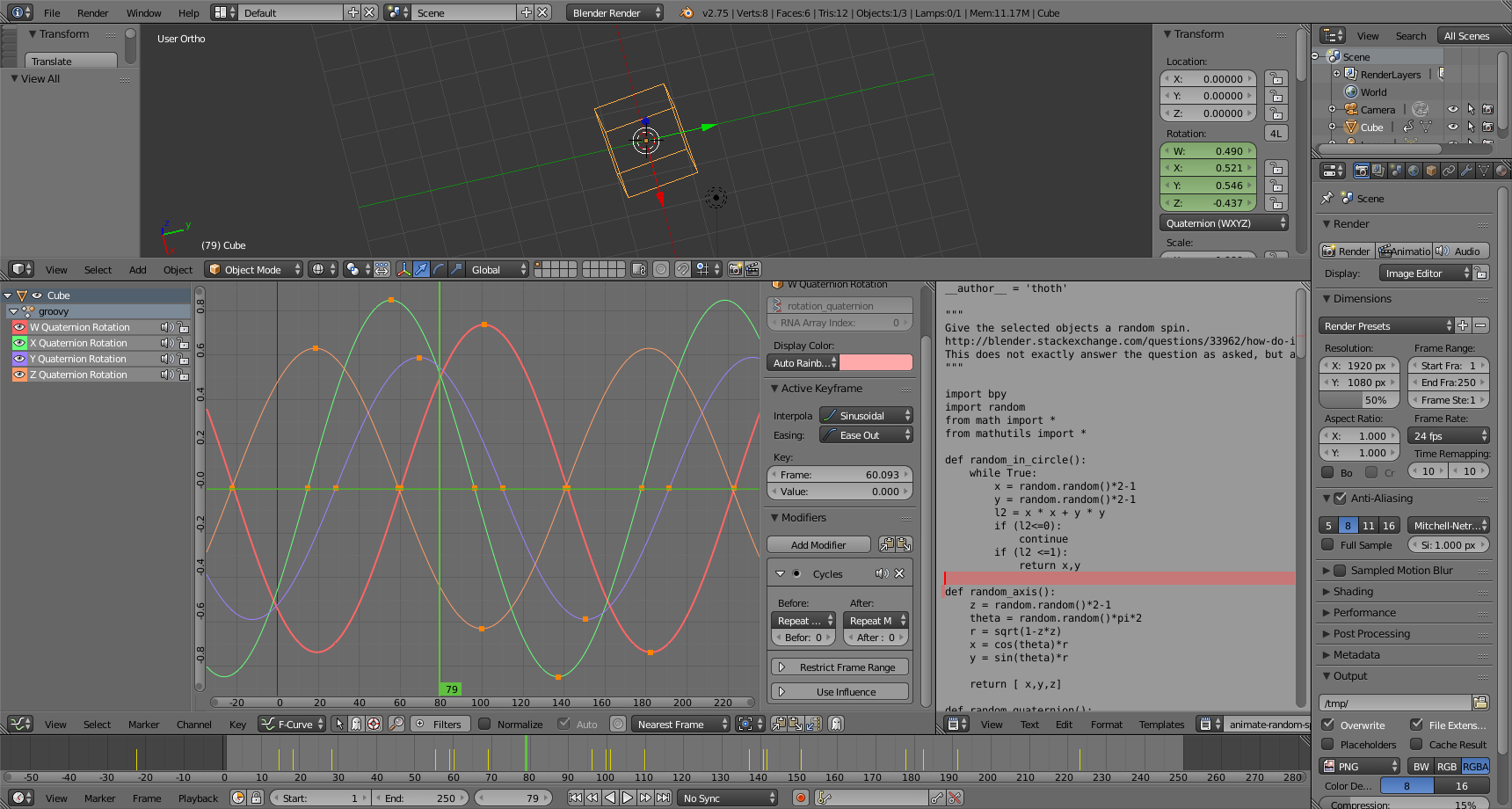
When we put this into practice with the animate-random-spin.py script we end up with fcurves that look like this:

How to keyframe a continuous rotation about a random axis in blender

or would we?

related links